How deep learning can represent War and Peace as a vector

Applications of neural networks have expanded significantly in recent years from image segmentation to natural language processing to time-series forecasting. One notably successful use of deep learning is embedding, a method used to represent discrete variables as continuous vectors. This technique has found practical applications with word embeddings for machine translation and entity embeddings for categorical variables.

In this article, I’ll explain what neural network embeddings are, why we want to use them, and how they are learned. We’ll go through these concepts in the context of a real problem I’m working on: representing all the books on Wikipedia as vectors to create a book recommendation system.

Neural Network Embedding of all books on Wikipedia. (From Jupyter Notebook on GitHub).

Embeddings

An embedding is a mapping of a discrete — categorical — variable to a vector of continuous numbers. In the context of neural networks, embeddings are low-dimensional, learned continuous vector representations of discrete variables. Neural network embeddings are useful because they can reduce the dimensionality of categorical variables and meaningfully represent categories in the transformed space.

Neural network embeddings have 3 primary purposes:

1. Finding nearest neighbors in the embedding space. These can be used to make recommendations based on user interests or cluster categories.
2. As input to a machine learning model for a supervised task.
3. For visualization of concepts and relations between categories.

This means in terms of the book project, using neural network embeddings, we can take all 37,000 book articles on Wikipedia and represent each one using only 50 numbers in a vector. Moreover, because embeddings are learned, books that are more similar in the context of our learning problem are closer to one another in the embedding space.

Neural network embeddings overcome the two limitations of a common method for representing categorical variables: one-hot encoding.

Limitations of One Hot Encoding

The operation of one-hot encoding categorical variables is actually a simple embedding where each category is mapped to a different vector. This process takes discrete entities and maps each observation to a vector of 0s and a single 1 signaling the specific category.

The one-hot encoding technique has two main drawbacks:

1. For high-cardinality variables — those with many unique categories — the dimensionality of the transformed vector becomes unmanageable.
2. The mapping is completely uninformed: “similar” categories are not placed closer to each other in embedding space.

The first problem is well-understood: for each additional category — referred to as an entity — we have to add another number to the one-hot encoded vector. If we have 37,000 books on Wikipedia, then representing these requires a 37,000-dimensional vector for each book, which makes training any machine learning model on this representation infeasible.

The second problem is equally limiting: one-hot encoding does not place similar entities closer to one another in vector space. If we measure similarity between vectors using the cosine distance, then after one-hot encoding, the similarity is 0 for every comparison between entities.

This means that entities such as War and Peace and Anna Karenina (both classic books by Leo Tolstoy) are no closer to one another than War and Peace is to The Hitchhiker’s Guide to the Galaxy if we use one-hot encoding.

# One Hot Encoding Categoricals
books = ["War and Peace", "Anna Karenina", 
          "The Hitchhiker's Guide to the Galaxy"]
books_encoded = [[1, 0, 0],
                 [0, 1, 0],
                 [0, 0, 1]]
Similarity (dot product) between First and Second = 0
Similarity (dot product) between Second and Third = 0
Similarity (dot product) between First and Third = 0

Considering these two problems, the ideal solution for representing categorical variables would require fewer numbers than the number of unique categories and would place similar categories closer to one another.

# Idealized Representation of Embedding
books = ["War and Peace", "Anna Karenina", 
          "The Hitchhiker's Guide to the Galaxy"]
books_encoded_ideal = [[0.53,  0.85],
                       [0.60,  0.80],
                       [-0.78, -0.62]]
Similarity (dot product) between First and Second = 0.99
Similarity (dot product) between Second and Third = -0.94
Similarity (dot product) between First and Third = -0.97

To construct a better representation of categorical entities, we can use an embedding neural network and a supervised task to learn embeddings.

Learning Embeddings

The main issue with one-hot encoding is that the transformation does not rely on any supervision. We can greatly improve embeddings by learning them using a neural network on a supervised task. The embeddings form the parameters — weights — of the network which are adjusted to minimize loss on the task. The resulting embedded vectors are representations of categories where similar categories — relative to the task — are closer to one another.

For example, if we have a vocabulary of 50,000 words used in a collection of movie reviews, we could learn 100-dimensional embeddings for each word using an embedding neural network trained to predict the sentimentality of the reviews. (For exactly this application see this Google Colab Notebook). Words in the vocabulary that are associated with positive reviews such as “brilliant” or “excellent” will come out closer in the embedding space because the network has learned these are both associated with positive reviews.

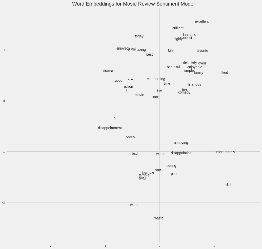Movie Sentiment Word Embeddings (source)

In the book example given above, our supervised task could be “identify whether or not a book was written by Leo Tolstoy” and the resulting embeddings would place books written by Tolstoy closer to each other. Figuring out how to create the supervised task to produce relevant representations is the toughest part of making embeddings.

Implementation

In the Wikipedia book project (complete notebook here), the supervised learning task is set as predicting whether a given link to a Wikipedia page appears in the article for a book. We feed in pairs of (book title, link) training examples with a mix of positive — true — and negative — false — pairs. This set-up is based on the assumption that books which link to similar Wikipedia pages are similar to one another. The resulting embeddings should therefore place alike books closer together in vector space.

The network I used has two parallel embedding layers that map the book and wikilink to separate 50-dimensional vectors and a dot product layer that combines the embeddings into a single number for a prediction. The embeddings are the parameters, or weights, of the network that are adjusted during training to minimize the loss on the supervised task.

In Keras code, this looks like the following (don’t worry if you don’t completely understand the code, just skip to the images):

Although in a supervised machine learning task the goal is usually to train a model to make predictions on new data, in this embedding model, the predictions can be just a means to an end. What we want is the embedding weights, the representation of the books and links as continuous vectors.

The embeddings by themselves are not that interesting: they are simply vectors of numbers:

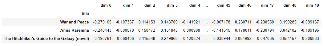Example Embeddings from Book Recommendation Embedding Model

However, the embeddings can be used for the 3 purposes listed previously, and for this project, we are primarily interested in recommending books based on the nearest neighbors. To compute similarity, we take a query book and find the dot product between its vector and those of all the other books. (If our embeddings are normalized, this dot product is the cosine distance between vectors that ranges from -1, most dissimilar, to +1, most similar. We could also use the Euclidean distance to measure similarity).

This is the output of the book embedding model I built:

Books closest to War and Peace.

Book: War and Peace              Similarity: 1.0
Book: Anna Karenina              Similarity: 0.79
Book: The Master and Margarita   Similarity: 0.77
Book: Doctor Zhivago (novel)     Similarity: 0.76
Book: Dead Souls                 Similarity: 0.75

(The cosine similarity between a vector and itself must be 1.0). After some dimensionality reduction (see below), we can make figures like the following:

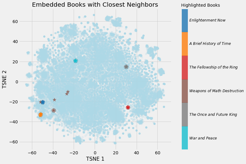Embedding Books with Closest Neighbors

We can clearly see the value of learning embeddings! We now have a 50-number representation of every single book on Wikipedia, with similar books closer to one another.

Embedding Visualizations

One of the coolest parts about embeddings are that they can be used to visualize concepts such as novel or non-fiction relative to one another. This requires a further dimension reduction technique to get the dimensions to 2 or 3. The most popular technique for reduction is itself an embedding method: t-Distributed Stochastic Neighbor Embedding (TSNE).

We can take the original 37,000 dimensions of all the books on Wikipedia, map them to 50 dimensions using neural network embeddings, and then map them to 2 dimensions using TSNE. The result is below:

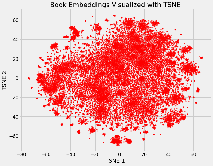Embedding of all 37,000 books on Wikipedia

(TSNE is a manifold learning technique which means that it tries to map high-dimensional data to a lower-dimensional manifold, creating an embedding that attempts to maintain local structure within the data. It’s almost exclusively used for visualization because the output is stochastic and it does not support transforming new data. An up and coming alternative is Uniform Manifold Approximation and Projection, UMAP, which is much faster and does support transform new data into the embedding space).

By itself this isn’t very useful, but it can be insightful once we start coloring it based on different book characteristics.

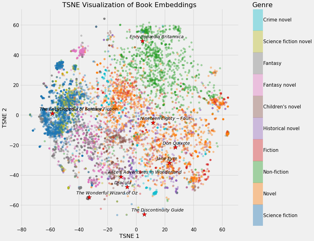
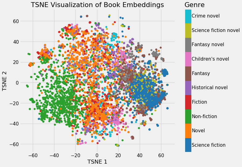Embeddings Colored by Genre

We can clearly see groupings of books belonging to the same genre. It’s not perfect, but it’s still impressive that we can represent all books on Wikipedia using just 2 numbers that still capture the variability between genres.

The book example (full article coming soon) shows the value of neural network embeddings: we have a vector representation of categorical objects that is both low-dimensional and places similar entities closer to one another in the embedded space.

Bonus: Interactive Visualizations

The problem with static graphs is that we can’t really explore the data and investigate groupings or relationships between variables. To solve this problem, TensorFlow developed projector, an online application that lets us visualize and interact with embeddings. I’ll release an article on how to use this tool shortly, but for now, here’s the results:

Interactive Exploration of Book Embeddings using projector

Conclusions

Neural network embeddings are learned low-dimensional representations of discrete data as continuous vectors. These embeddings overcome the limitations of traditional encoding methods and can be used for purposes such as finding nearest neighbors, input into another model, and visualizations.

Although many deep learning concepts are talked about in academic terms, neural network embeddings are both intuitive and relatively simple to implement. I firmly believe that anyone can learn deep learning and use libraries such as Keras to build deep learning solutions. Embeddings are an effective tool for handling discrete variables and present a useful application of deep learning.

Resources

• Google-Produced tutorial on embeddings
• TensorFlow Guide to Embeddings
• Book Recommendation System Using Embeddings
• Tutorial on Word Embeddings in Keras

As always, I welcome feedback and constructive criticism. I can be reached on Twitter @koehrsen_will or on my personal website at willk.online.